预处理数据
1. 获取数据
获取 2009~2016 年的数据。
zip_path = tf.keras.utils.get_file(
    origin='https://storage.googleapis.com/tensorflow/tf-keras-datasets/jena_climate_2009_2016.csv.zip',
    fname='jena_climate_2009_2016.csv.zip',
    extract=True)
csv_path, _ = os.path.splitext(zip_path)
将其由 10 分钟的数据截取为 1 小时的数据。
df = pd.read_csv(csv_path)
# slice [start:stop:step], starting from index 5 take every 6th record.
df = df[5::6]

date_time = pd.to_datetime(df.pop('Date Time'), format='%d.%m.%Y %H:%M:%S')
print(df.head())| p (mbar) | T (degC) | Tpot (K) | Tdew (degC) | rh (%) | VPmax (mbar) | VPact (mbar) | VPdef (mbar) | sh (g/kg) | H2OC (mmol/mol) | rho (g/m**3) | wv (m/s) | max. wv (m/s) | wd (deg) | |
|---|---|---|---|---|---|---|---|---|---|---|---|---|---|---|
| 5 | 996.5 | -8.05 | 265.38 | -8.78 | 94.4 | 3.33 | 3.14 | 0.19 | 1.96 | 3.15 | 1307.86 | 0.21 | 0.63 | 192.7 |
| 11 | 996.62 | -8.88 | 264.54 | -9.77 | 93.2 | 3.12 | 2.9 | 0.21 | 1.81 | 2.91 | 1312.25 | 0.25 | 0.63 | 190.3 |
| 17 | 996.84 | -8.81 | 264.59 | -9.66 | 93.5 | 3.13 | 2.93 | 0.2 | 1.83 | 2.94 | 1312.18 | 0.18 | 0.63 | 167.2 |
| 23 | 996.99 | -9.05 | 264.34 | -10.02 | 92.6 | 3.07 | 2.85 | 0.23 | 1.78 | 2.85 | 1313.61 | 0.1 | 0.38 | 240 |
| 29 | 997.46 | -9.63 | 263.72 | -10.65 | 92.2 | 2.94 | 2.71 | 0.23 | 1.69 | 2.71 | 1317.19 | 0.4 | 0.88 | 157 |
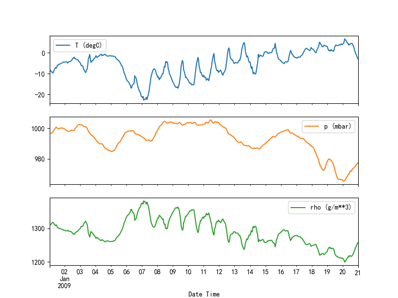
2. 数据间的关系
这里展示 T (degC) , p (mbar) , rho (g/m**3) 和 Date Time 之间的关系。
plot_cols = ['T (degC)', 'p (mbar)', 'rho (g/m**3)']
plot_features = df[plot_cols]
plot_features.index = date_time
_ = plot_features.plot(subplots=True)
plt.draw()

plot_features = df[plot_cols][:480]
plot_features.index = date_time[:480]
_ = plot_features.plot(subplots=True)
plt.draw()

plt.show()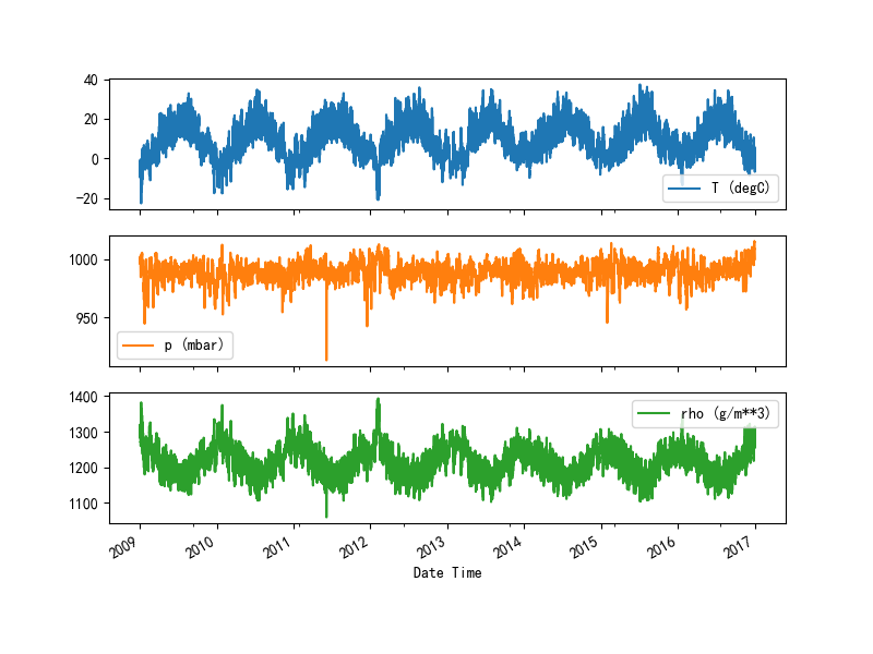
3. 检查和清理数据 Inspect and cleanup
print(df.describe().transpose())| count | mean | std | min | 25% | 50% | 75% | max | |
|---|---|---|---|---|---|---|---|---|
| p (mbar) | 70091 | 989.21284 | 8.358886 | 913.6 | 984.2 | 989.57 | 994.72 | 1015.29 |
| T (degC) | 70091 | 9.450482 | 8.423384 | -22.76 | 3.35 | 9.41 | 15.48 | 37.28 |
| Tpot (K) | 70091 | 283.49309 | 8.504424 | 250.85 | 277.44 | 283.46 | 289.53 | 311.21 |
| Tdew (degC) | 70091 | 4.956471 | 6.730081 | -24.8 | 0.24 | 5.21 | 10.08 | 23.06 |
| rh (%) | 70091 | 76.009788 | 16.47492 | 13.88 | 65.21 | 79.3 | 89.4 | 100 |
| VPmax (mbar) | 70091 | 13.576576 | 7.739883 | 0.97 | 7.77 | 11.82 | 17.61 | 63.77 |
| VPact (mbar) | 70091 | 9.533968 | 4.183658 | 0.81 | 6.22 | 8.86 | 12.36 | 28.25 |
| VPdef (mbar) | 70091 | 4.042536 | 4.898549 | 0 | 0.87 | 2.19 | 5.3 | 46.01 |
| sh (g/kg) | 70091 | 6.02256 | 2.655812 | 0.51 | 3.92 | 5.59 | 7.8 | 18.07 |
| H2OC (mmol/mol) | 70091 | 9.640437 | 4.234862 | 0.81 | 6.29 | 8.96 | 12.49 | 28.74 |
| rho (g/m**3) | 70091 | 1216.0612 | 39.974263 | 1059.45 | 1187.47 | 1213.8 | 1242.765 | 1393.54 |
| wv (m/s) | 70091 | 1.702567 | 65.447512 | -9999 | 0.99 | 1.76 | 2.86 | 14.01 |
| max. wv (m/s) | 70091 | 2.963041 | 75.597657 | -9999 | 1.76 | 2.98 | 4.74 | 23.5 |
| wd (deg) | 70091 | 174.7891 | 86.619431 | 0 | 125.3 | 198.1 | 234 | 360 |
这里发现 wv (m/s) 和 max. wv (m/s) 中的最小值为 -9999.00 。这可能是个错误,因为存在风向列 wd (deg) 所以值应该 >=0 。那么用零来替换它。
wv = df['wv (m/s)']
bad_wv = wv == -9999.0
wv[bad_wv] = 0.0

max_wv = df['max. wv (m/s)']
bad_max_wv = max_wv == -9999.0
max_wv[bad_max_wv] = 0.0

# The above inplace edits are reflected in the DataFrame
# 检验下最小值
df['wv (m/s)'].min()
4. 特征工程 Feature engineering
将特征进行一些转换使其格式更加合理。
4.1. 风 Wind
例如上面的风向 wd (deg) 为度数,取值范围 0~360。但是实际情况是 0° 和 360° 是同一个点。
我们将风向和风速绘制成图如下:
plt.figure()
plt.hist2d(df['wd (deg)'], df['wv (m/s)'], bins=(50, 50), vmax=400)
plt.colorbar()
plt.xlabel('Wind Direction [deg]')
plt.ylabel('Wind Velocity [m/s]')
plt.draw()

plt.show()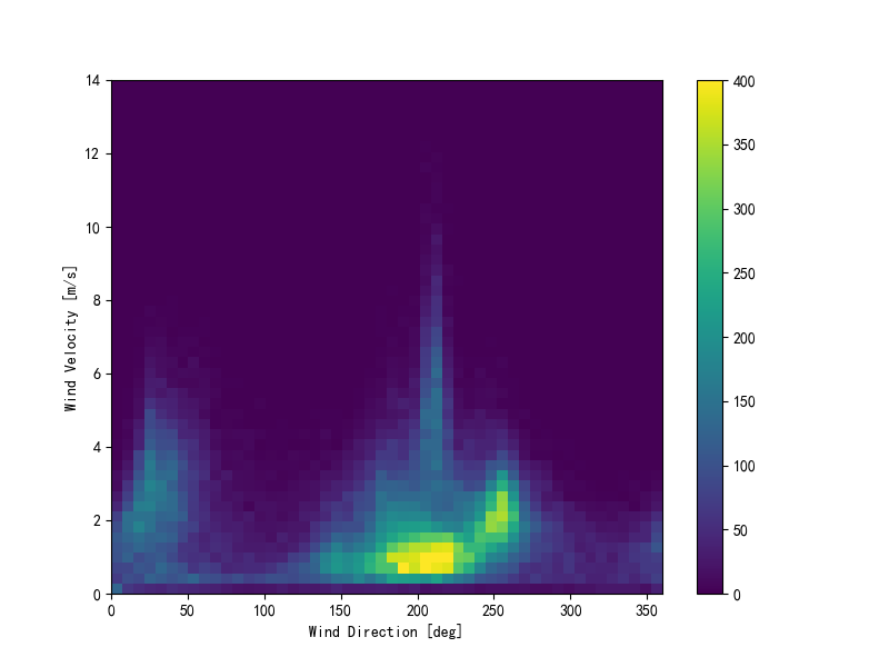
这里如果将风向和风速转化为矢量,那么模型就会更加容易理解这个数据了:
wv = df.pop('wv (m/s)')
max_wv = df.pop('max. wv (m/s)')

# Convert to radians. 转为弧度
wd_rad = df.pop('wd (deg)')*np.pi / 180

# Calculate the wind x and y components. 计算风的x和y分量。
df['Wx'] = wv*np.cos(wd_rad)
df['Wy'] = wv*np.sin(wd_rad)

# Calculate the max wind x and y components. 计算最大风x和y分量。
df['max Wx'] = max_wv*np.cos(wd_rad)
df['max Wy'] = max_wv*np.sin(wd_rad)
再次绘制风向和风速的关系图:
plt.figure()
plt.hist2d(df['Wx'], df['Wy'], bins=(50, 50), vmax=400)
plt.colorbar()
plt.xlabel('Wind X [m/s]')
plt.ylabel('Wind Y [m/s]')
ax = plt.gca()
ax.axis('tight')
plt.draw()

plt.show()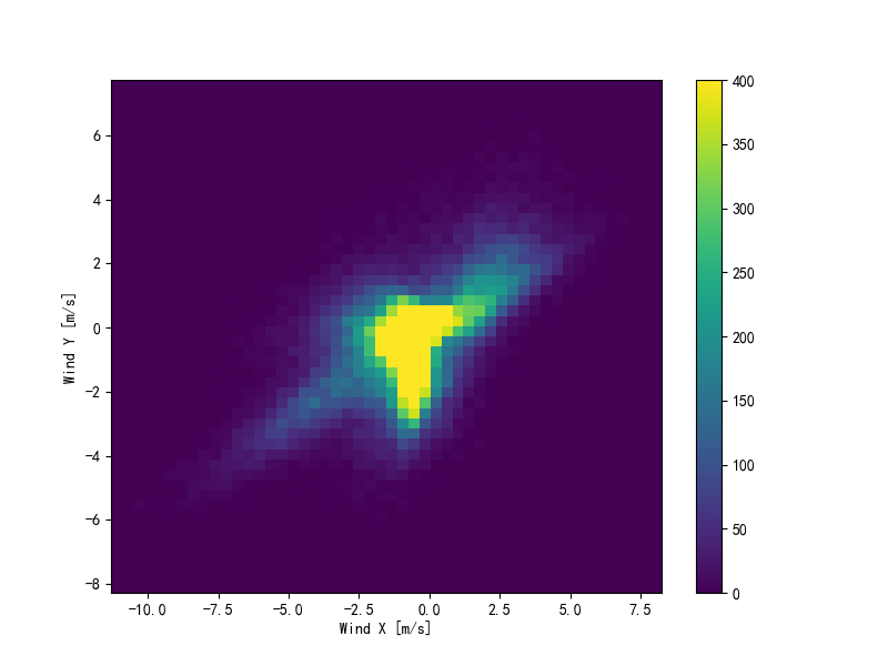
4.2. 时间 Time
相同的,Date Time 列也有很大的作用,但是它目前是字符串形式的,我们需要将它转化为秒的形式:
timestamp_s = date_time.map(datetime.datetime.timestamp)与风向类似,以秒为单位的时间也不是一个有效的模型输入。作为气象资料,具有明显的周期性,例如日、年等。有很多方式可以处理周期性数据。将其转换为可用数据的最简单的方式是使用 sin 和 cos 将时间转换为明确的周期数据。
day = 24*60*60
year = (365.2425)*day

df['Day sin'] = np.sin(timestamp_s * (2 * np.pi / day))
df['Day cos'] = np.cos(timestamp_s * (2 * np.pi / day))
df['Year sin'] = np.sin(timestamp_s * (2 * np.pi / year))
df['Year cos'] = np.cos(timestamp_s * (2 * np.pi / year))

plt.figure()
plt.plot(np.array(df['Day sin'])[:25])
plt.plot(np.array(df['Day cos'])[:25])
plt.xlabel('Time [h]')
plt.title('Time of day signal')
plt.draw()

plt.show()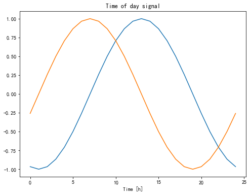
这样就能使得模型很容易的理解频率这个重要特征了。但是这种是在你提前知道哪些频率是重要的情况下才能如此操作。
如果你不知道频率,你可以使用 fft 来确定哪些频率是重要的。为了检验我们的假设(日和年),我们使用 tf.signal.rfft 来查看温度随时间的变化。注意在 1/day 和 1/year 附近有明显的峰值:
fft = tf.signal.rfft(df['T (degC)'])
f_per_dataset = np.arange(0, len(fft))

n_samples_h = len(df['T (degC)'])
hours_per_year = 24*365.2524
years_per_dataset = n_samples_h/(hours_per_year)

f_per_year = f_per_dataset/years_per_dataset

plt.figure()
plt.step(f_per_year, np.abs(fft))
plt.xscale('log')
plt.ylim(0, 400000)
plt.xlim([0.1, max(plt.xlim())])
plt.xticks([1, 365.2524], labels=['1/Year', '1/day'])
_ = plt.xlabel('Frequency (log scale)')
plt.draw()

plt.show()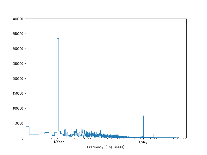
5. 分割数据 Split the data
- 训练集 training sets:70%
- 验证集 validation sets:20%
- 测试集 test sets:10%
注意:数据在分割前并没有被随机打乱。这有两个原因。
- 确保将数据切成连续样本的窗口仍然是可能的。
- 通过对模型训练后收集的数据进行评估,确保验证/测试结果更加真实。
column_indices = {name: i for i, name in enumerate(df.columns)}

n = len(df)
train_df = df[0:int(n*0.7)]
val_df = df[int(n*0.7):int(n*0.9)]
test_df = df[int(n*0.9):]

num_features = df.shape[1]
6. 归一化/标准化数据 Normalize the data
在训练神经网络之前,对特征进行缩放是很重要的。标准化是进行缩放的常用方法。减去平均值,然后除以每个特征的标准差。
平均值和标准偏差应该只使用训练数据进行计算,这样模型就无法访问到验证和测试集中的值。
在训练时,模型不应该访问训练集中的未来的值,这种归一化应该使用移动平均。这不是本教程的重点,验证和测试集确保您获得(某种程度上)真实的度量。为了简单起见,本教程使用了一个简单的平均值。
train_mean = train_df.mean()  # 平均值
train_std = train_df.std()  # 标准差

train_df = (train_df - train_mean) / train_std
val_df = (val_df - train_mean) / train_std
test_df = (test_df - train_mean) / train_std
现在来看看这些特性的分布。有些特征确实有长尾,但没有明显的错误,如-9999 风速值。
df_std = (df - train_mean) / train_std
df_std = df_std.melt(var_name='Column', value_name='Normalized')
plt.figure(figsize=(12, 6))
ax = sns.violinplot(x='Column', y='Normalized', data=df_std)
_ = ax.set_xticklabels(df.keys(), rotation=90)
plt.draw()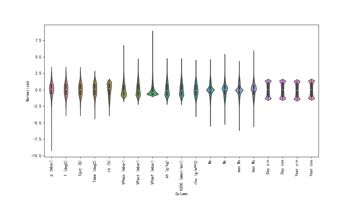
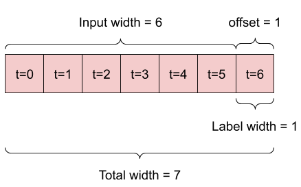
7. 数据窗口 Data windowing
一个方便处理连续样本的窗口。
输入:
- 输入数据的宽度和预测数据的宽度
- 输入和输出之间的偏移量
- 哪些特征作为输入、标签。
本教程构建了各种模型,并将他们用于:
- 单输出和多输出的预测。
- 单时间步长和多时间步长预测。
下面是两个例子:
- 给定 24 小时数据,预测未来 24 小时时的数据:

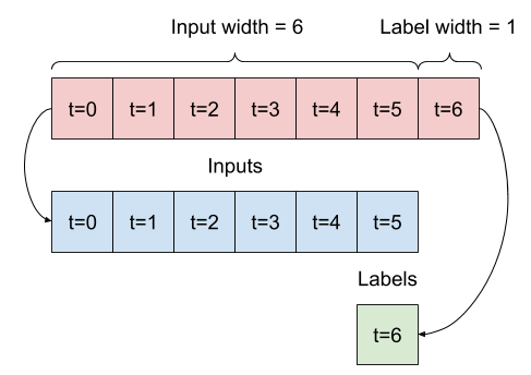
- 给定 6 小时的数据,预测未来 1 小时的数据:
class WindowGenerator():
    def __init__(self, input_width, label_width, shift,
                 train_df=train_df, val_df=val_df, test_df=test_df,
                 label_columns=None):
        # Store the raw data. 存储原始数据。
        self.train_df = train_df
        self.val_df = val_df
        self.test_df = test_df

        # Work out the label column indices. 计算出标签列索引。
        self.label_columns = label_columns
        if label_columns is not None:
            self.label_columns_indices = {name: i for i, name in
                                          enumerate(label_columns)}
        self.column_indices = {name: i for i, name in
                               enumerate(train_df.columns)}

        # Work out the window parameters. 计算出窗口参数。
        self.input_width = input_width
        self.label_width = label_width
        self.shift = shift

        self.total_window_size = input_width + shift

        self.input_slice = slice(0, input_width)
        self.input_indices = np.arange(self.total_window_size)[
            self.input_slice]

        self.label_start = self.total_window_size - self.label_width
        self.labels_slice = slice(self.label_start, None)
        self.label_indices = np.arange(self.total_window_size)[
            self.labels_slice]

    def __repr__(self):
        return '\n'.join([
            f'Total window size: {self.total_window_size}',
            f'Input indices: {self.input_indices}',
            f'Label indices: {self.label_indices}',
            f'Label column name(s): {self.label_columns}'])
上面两个的定义分别为:
w1 = WindowGenerator(input_width=24, label_width=1, shift=24, label_columns=['T (degC)'])
w2 = WindowGenerator(input_width=6, label_width=1, shift=1, label_columns=['T (degC)'])
print(w1)
print(w2)
7.1. 分割数据
将连续的输入列表通过 split_window 方法将他们转化为输入和标签。
上面的 w2 将像这样进行拆分:
def split_window(self, features):
    inputs = features[:, self.input_slice, :]
    labels = features[:, self.labels_slice, :]
    if self.label_columns is not None:
        labels = tf.stack(
            [labels[:, :, self.column_indices[name]]
                for name in self.label_columns],
            axis=-1)

    # Slicing doesn't preserve static shape information, so set the shapes
    # manually. This way the `tf.data.Datasets` are easier to inspect.
    # 切片不会保留静态shape信息,所以要手动设置shape。这样`tf.data.Datasets`更容易检查。
    inputs.set_shape([None, self.input_width, None])
    labels.set_shape([None, self.label_width, None])

    return inputs, labels


WindowGenerator.split_window = split_window最后更新: 2022-07-30 02:00:00